The works of François Morellet

library(sf)
library(dplyr)
library(ggplot2)
library(tidyr)

sf_use_s2(FALSE)

I’ve not posted much this year by comparison with last, and have come to the conclusion that I was posting too often for it to be sustainable.

This post is a palette cleanser before getting back into the habit at a more sustainable pace. So, “who is Francois Morellet?” I hear you ask. I’ll save you the trouble of checking out the Wikipedia entry, which has this to say:

François Morellet (30 April 1926 – 10 May 2016) was a French contemporary abstract painter, sculptor, and light artist. His early work prefigured minimal art and conceptual art and he played a prominent role in the development of geometrical abstract art and post-conceptual art. There’s much more at his website, where the breadth of his work over a long career is apparent, although you’ll have to visit his instagram for more pretty pictures.

What’s this got to do with geospatial stuff? Well, for several years, I would use the work Random Distribution of 40,000 Squares Using the Odd and Even Numbers of a Telephone Directory, 50% Blue, 50% Red as my beginner example of a spatial process. The Museum of Modern Art description spells it out:

For this work, he divided the canvas into a grid of forty thousand squares, then instructed his wife or his sons to read numbers from the phone book out loud. Moving from the top left corner of the canvas to the bottom right, he marked a square for each even number and skipped a square for each odd one. Upon reaching the end, he colored the marked squares blue and the blank ones red.

A spatial process no less! As is often the case with this sort of thing, the indication in the title that half the squares are blue and half are red leaves the exact method of construction a little unclear. But it’s easy to make a version in R:

two_states <- expand_grid(x = 1:200, y = 1:200) |>
  mutate(colour = rep(c(TRUE, FALSE), 20000) |> sample(40000))

ggplot(two_states) +
  geom_raster(aes(x = x, y = y, fill = colour)) +
  scale_fill_manual(values = c("#ff3333", "#3333ff")) +
  coord_equal(expand = FALSE) +
  guides(fill = "none") +
  theme_void()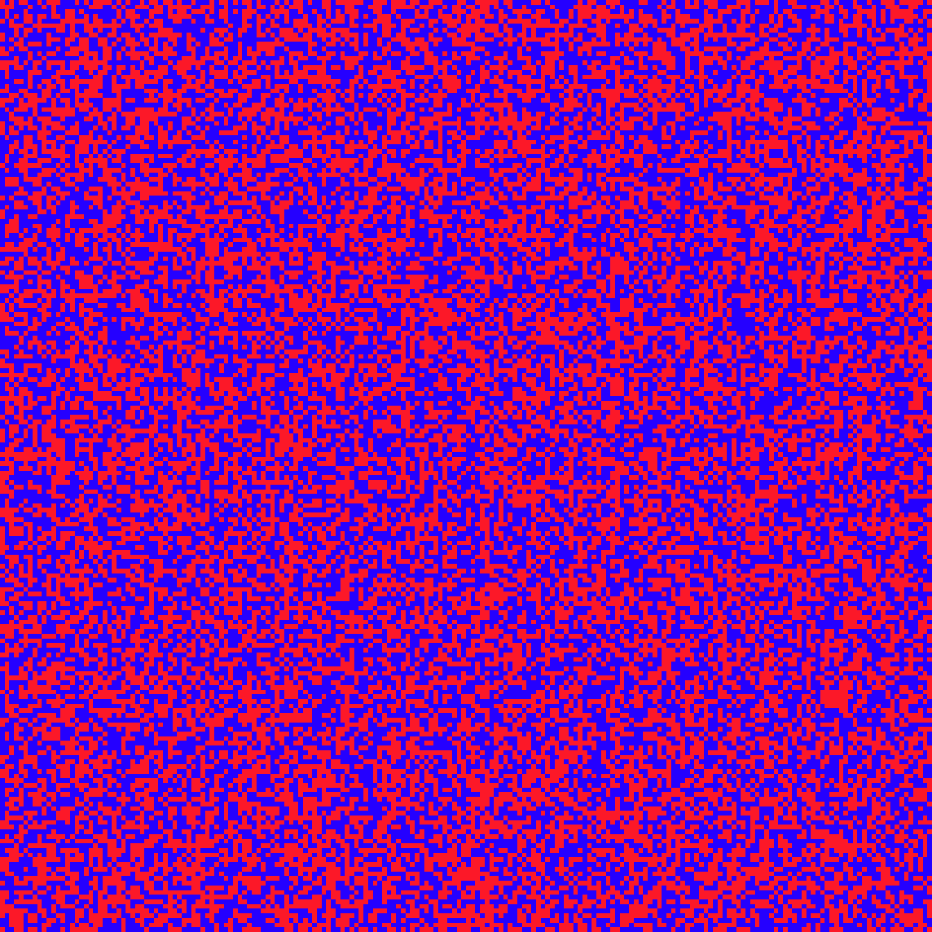

Figure 1: A version of Random Distribution of 40,000 Squares Using the Odd and Even Numbers of a Telephone Directory, 50% Blue, 50% Red

And so it begins… I was revisiting this example, as I started to put together a post on spatial processes for my stalled series of posts on materials supporting Geographic Information Analysis a François Morellet rabbit hole opened up before me, and I jumped in. There follow four more works by the great man, rendered in R.

Some helper functions

In what follows we use simple sf shapes and rotations and translations of them, so some helper functions for making and manipulating them are useful.

get_square <- function() {
  st_polygon(list(matrix(
    c(-1, 1, 1, -1, -1, -1, -1, 1, 1, -1) * 0.5,
    ncol = 2
  )))
}

get_rectangle <- function(width, height) {
  get_square() * matrix(c(width, 0, 0, height), 2, 2)
}

rotate_shape <- function(s, angle) {
  a <- -pi / 180 * angle
  s * matrix(c(cos(a), sin(a), -sin(a), cos(a)), 2, 2)
}

translate_shape <- function(s, dx, dy) {
  s + c(dx, dy)
}

get_l_shape <- function(size = 100) {
  st_linestring(matrix(c(size, 0, 0, 0, 0, size), ncol = 2))
}

Four prints from Album de 10 sérigraphies sur 10 ans

16 Carrés

Although the title of this work in English is 16 Squares it is more conveniently produced using geom_hline and geom_vline:

ggplot() +
  geom_hline(aes(yintercept = 1:3), lwd = 0.75) +
  geom_vline(aes(xintercept = 1:3), lwd = 0.75) +
  coord_equal(
    xlim = c(0, 4),
    ylim = c(0, 4), expand = FALSE
  ) +
  theme_void()

Figure 2: A version of 16 Carrées

Title uncertain: 34 lines or rectangles?

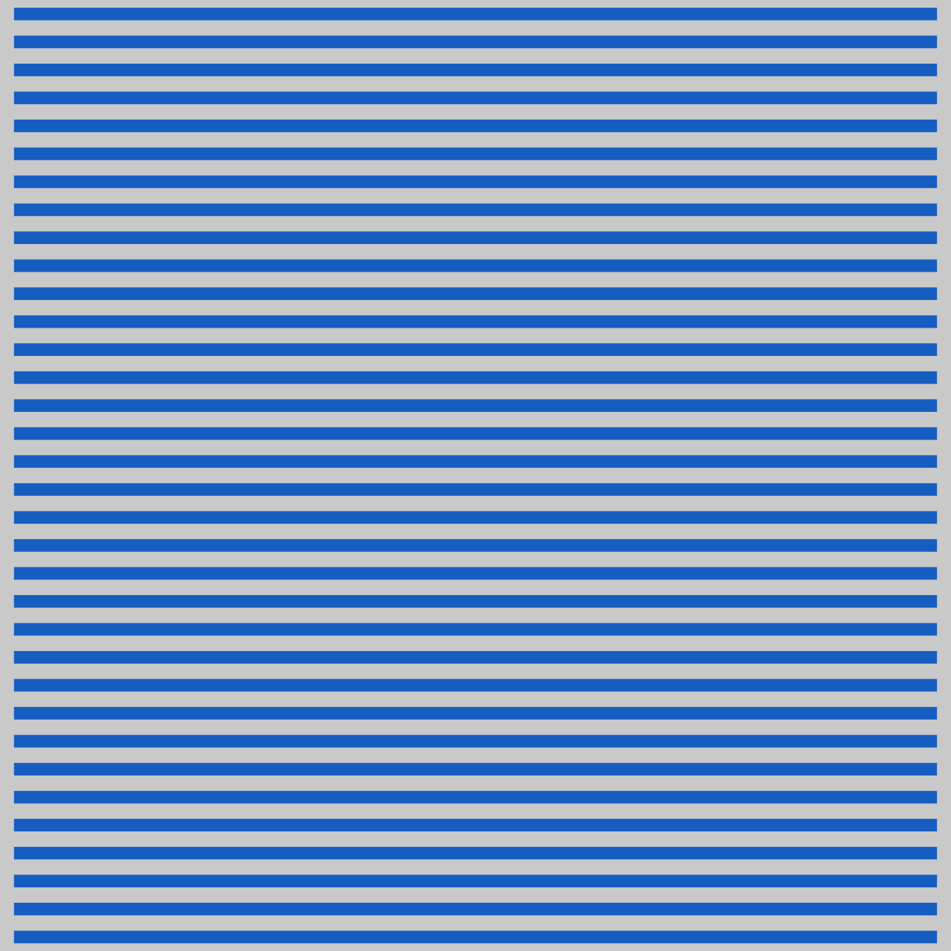
This one might also be realised using geom_hline like this:

ggplot() +
  geom_hline(aes(yintercept = 0:33 - 16.5),
    colour = "dodgerblue3", lwd = 2.4
  ) +
  coord_equal(
    xlim = c(-17, 17),
    ylim = c(-17, 17), expand = FALSE
  ) +
  theme_void() +
  theme(
    panel.background = element_rect(fill = "lightgrey", colour = NA)
  )

Figure 3: 34 Lines

But given the thickness of the ‘lines’ perhaps they are better considered rectangles.

s <- get_rectangle(33, 0.45)
rectangles <- list()
for (i in 1:34) {
  rectangles[[i]] <- translate_shape(s, 0, i - 17.5)
}
rectangles <- rectangles |>
  st_as_sfc() |>
  data.frame() |>
  st_sf()

ggplot() +
  geom_sf(
    data = rectangles,
    fill = "dodgerblue3", colour = NA
  ) +
  coord_sf(
    xlim = c(-17, 17),
    ylim = c(-17, 17), expand = FALSE
  ) +
  theme_void() +
  theme(
    panel.background = element_rect(fill = "lightgrey", colour = NA)
  )

Figure 4: 34 Rectangles

Title uncertain: 32 right angles?

This work seems to be most easily realised as a set of right-angle L shapes rotated and translated appropriately.

L1 <- get_l_shape() |> rotate_shape(-45)
L2 <- rotate_shape(L1, 90)
L3 <- rotate_shape(L2, 90)
L4 <- rotate_shape(L3, 90)
l_shapes <- list()
for (d in 0.25 + (0:7) / 2) {
  l_shapes[[length(l_shapes) + 1]] <- translate_shape(L1, d, 0)
  l_shapes[[length(l_shapes) + 1]] <- translate_shape(L2, 0, d)
  l_shapes[[length(l_shapes) + 1]] <- translate_shape(L3, -d, 0)
  l_shapes[[length(l_shapes) + 1]] <- translate_shape(L4, 0, -d)
}
lims <- c(-4, 4)
l_shapes <- l_shapes |>
  st_as_sfc() |>
  data.frame() |>
  st_sf() |>
  st_intersection(get_square() * lims[2] * 2)

ggplot() +
  geom_sf(data = l_shapes, fill = NA, colour = "black") +
  coord_sf(xlim = c(-4, 4), ylim = c(-4, 4), expand = FALSE) +
  theme_void()

Figure 5: 32 Right Angles

Title uncertain: red roof contours?

Finally, and most interesting, I think, (shades of Bridget Riley in the way it messes with the flatness of the plane) is this work. Red roof contours might not be quite right, but it feels like it could be.

I initially made this by buffering a bunch of squares, and moving them around as required, but on reflection, a cleaner method is based again on L shapes. It was tricky to position the squares correctly to get the vertical offset between the two sides of the picture. This became a lot easier using L shapes.

offset <- 20
lims <- c(-1, 1) * (3 * offset + 0.1)
spacing <- 2

L1 <- get_l_shape() |>
  translate_shape(0, offset)
L2 <- get_l_shape() |>
  rotate_shape(-90) |>
  translate_shape(0, offset)

l_shapes <- list(L2)
for (i in 1:100) {
  l_shapes[[length(l_shapes) + 1]] <-
    translate_shape(L1, spacing * i, spacing * i)
  l_shapes[[length(l_shapes) + 1]] <-
    translate_shape(L2, spacing * i, -spacing * i)
}
l_shapes_2 <- lapply(l_shapes, rotate_shape, angle = 180)

l_shapes <- l_shapes |>
  append(l_shapes_2) |>
  st_as_sfc() |>
  data.frame() |>
  st_sf() |>
  st_intersection(get_square() * lims[2] * 2)

ggplot() +
  geom_sf(data = l_shapes, fill = NA, colour = "red", lwd = spacing) +
  coord_sf(xlim = lims, ylim = lims, expand = FALSE) +
  theme_void()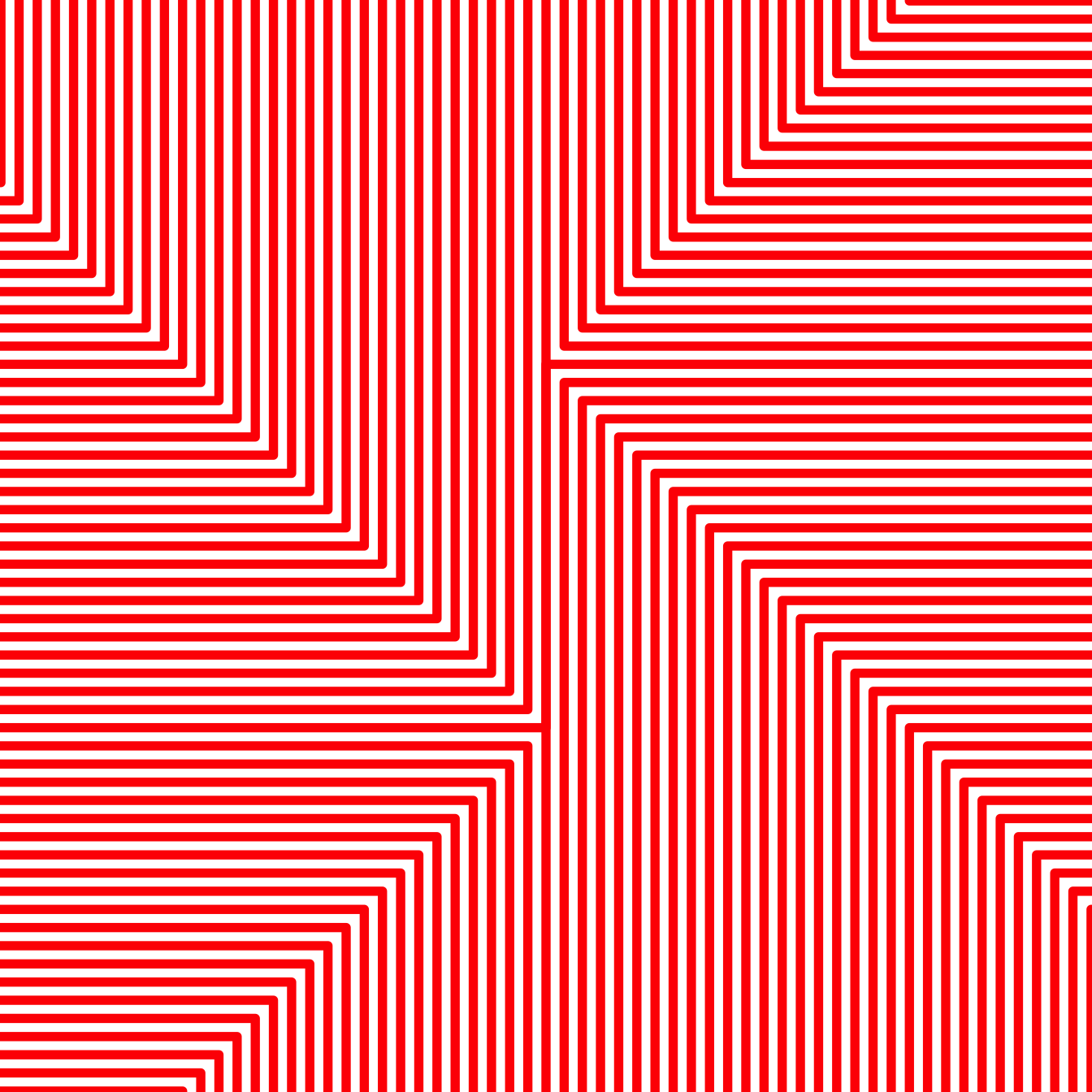

Figure 6: Red Roof Contours

This has been fun, if not especially productive. Definitely a theme worth returning.