Code
import math

import geopandas as gpd
import matplotlib.pyplot as plt
from shapely import geometry as geom

import weavingspace as wspimport math
import geopandas as gpd
import matplotlib.pyplot as plt
from shapely import geometry as geom
import weavingspace as wspWhen I’m not doing real work, a major side-project for me in the last couple of years has been developing and maintaining the weavingspace python module for making tiled maps of multivariate data.
An intermittently rewarding aspect to this has been finding cool1 tilings and implementing them as part of the _tiling_geometries.py source file in weavingspace. I can write the function to setup a new tiling while watching television these days, because the essentials of the required code are basically the same each time. But as that file has grown to 2000+ lines of ad hoc code, I’ve had a nagging sense that there must be a more coherent way to represent and generate tilings; if not all tilings then at least those composed of regular polygons. These are the ones where I find myself making a bunch of polygons, then translating and rotating them into position to form the set of repeating elements required by weavingspace, and in the process reusing lots of almost-but-not-quite identical chunks of code, over and over.
Anyway, a week or so ago I came across a really smart project based around a compact, integer-based representation of such tilings. The paper explaining the work is
Soto Sánchez JE, T Weyrich, A Medeiros e Sá, and LH de Figueiredo. 2021. An integer representation for periodic tilings of the plane by regular polygons. Computers & Graphics 95 69-80. doi: 10.1016/j.cag.2021.01.007.
The approach has a reference implementation in Javascript2, which I had to trans-code into Python3 for use in weavingspace. The net result is that the experimental branch of weavingspace now offers 1500 or so regular tilings, should anyone ever want to use them.4
In this post, I am here to share my (admittedly niche) enthusiasm about this approach, along with some relevant code. It’s a real lesson in how the right representation can make a challenging programming problem much simpler. The code included below is lightly modified from the reasonably well commented code in this notebook in the experimental branch of weavingspace. Also included there, and my own contribution is generation of the corresponding dual tilings.
A couple of convenience functions for element-wise summing and multiplying vectors, along with functions to generate points, lines, and polygons for illustrative purposes along the way. It’s a bit of a sledgehammer using shapely, and geopandas here for handling points, lines, and polygons, but it saves a lot of faffing around setting the aspect ratios of plots and so forth.
def vsum(*a):
  return tuple(sum(_) for _ in zip(*a, strict = True))

def vprod(*a):
  if isinstance(a[0], float|int):
    return tuple(a[0] * math.prod(_) for _ in zip(*a[1:], strict = True))
  return tuple(math.prod(_) for _ in zip(*a, strict = True))

def to_euclidean(coords):
  return sum(vprod(coords, DX)), sum(vprod(coords, DY))

def get_line(v, origin = (0, 0, 0, 0)):
  return geom.LineString([to_euclidean(origin), to_euclidean(vsum(origin, v))])

def get_point(v):
  return geom.Point(to_euclidean(v))

def get_polygon(vs):
  return geom.Polygon([get_point(v) for v in vs])
The key insight behind the approach is that in tilings by regular 3, 4, 6, and 12 sided polygons with equal-length sides, there are only 12 possible sides, which we here consider to be unit vectors. Given a particular orientation of the tiling, every polygon side will be in of only 12 orientations, and by definition all the sides are the same length. As an example, look carefully at the tiling below.
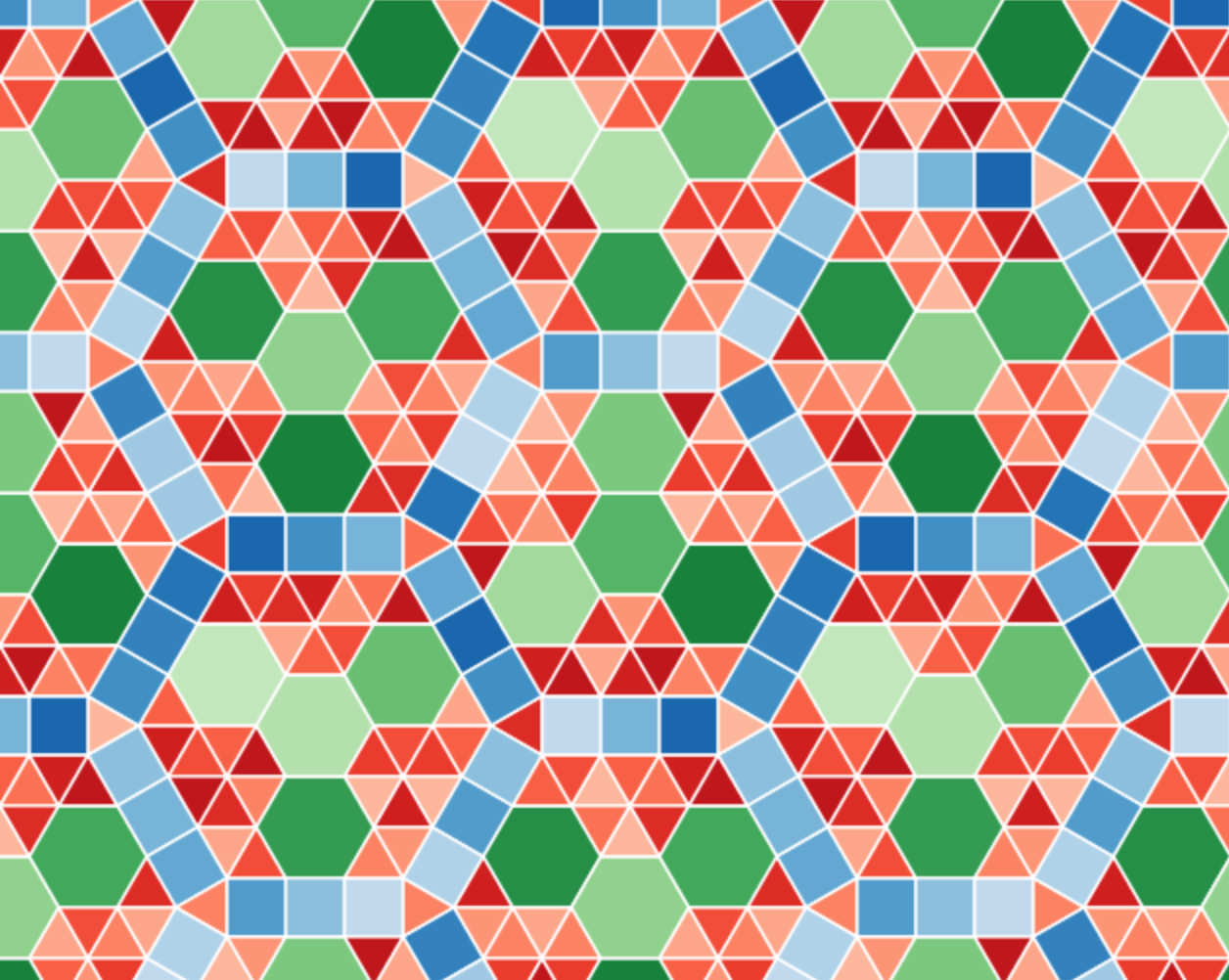
In spite of its complexity only 12 different tile edge orientations appear anywhere in this pattern. The pattern is dominated by edges parallel to the hexagonal tile edges, but six additional orientations appear in the blue squares that trace out the larger hexagonal structures.
This means that using only a set of unit vectors with orientations equally spaced at 30º intervals, we can trace out all the edges in this tiling, something that turns out to be true for all tilings composed of these regular polygons.5
Furthermore, we can encode the 12 vectors as 4 element integer vectors, because we only need linear combinations of the first four vectors at 0º, 30º, 60º, and 90º to the positive \(x\)-axis to generate any of the others.
These ideas give rise to the code below, where we have the four base vectors stored in the DXand DY tuples, and the combinations of the first four vectors to yield any of the 12 directions encoded as 4-tuples in BASE_COORDS.
DX = 1, 3 ** 0.5 / 2,          0.5, 0
DY = 0,          0.5, 3 ** 0.5 / 2, 1

# Coordinates of the twelve 30º spaced unit vectors expressed as combinations
# of 0, 30, 60, and 90º unit vectors. The first four are a single instance each
# of the four unit vectors. The other are linear combinations of these four.
BASE_COORDS = [
  ( 1,  0,  0,  0), ( 0,  1,  0,  0), ( 0,  0,  1,  0),
  ( 0,  0,  0,  1), (-1,  0,  1,  0), ( 0, -1,  0,  1),
  (-1,  0,  0,  0), ( 0, -1,  0,  0), ( 0,  0, -1,  0),
  ( 0,  0,  0, -1), ( 1,  0, -1,  0), ( 0,  1,  0, -1),
]
And here are the resulting twelve unit vectors:
basis = gpd.GeoSeries(
  [get_line(v) for v in BASE_COORDS])
ax = basis.plot(color = "k", lw = 0.5)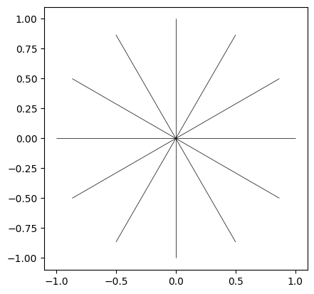
And, as an example of how they can be reduced to only combinations of the four vectors in the upper right quadrant, BASE_COORDS[4] being (-1, 0, 1, 0) tells us that the fifth unit vector, at 120º to the \(x\)-axis, is formed by combining the inverse (-1) of the first unit vector parallel to the \(x\)-axis, with the third unit (1) vector at 60º to the \(x\)-axis, as illustrated by the dotted red line below.
ax = basis.plot(lw = 0.35, color = "k")
gpd.GeoSeries([get_line(BASE_COORDS[2])]) \
  .plot(ax = ax, color = "r", ls = ":")
gpd.GeoSeries([get_line((-x for x in BASE_COORDS[0]), BASE_COORDS[2])]) \
  .plot(ax = ax, color = "r", ls = ":")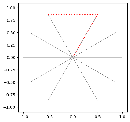
The sixth unit vector can be similarly encode, and the remaining six unit vectors are the inverse of the first six, derived by simply negating each coordinate in the corresponding 4-tuple (e.g., the 8th vector (0, -1, 0, 0) is the negative of the 2nd (0, 1, 0, 0).
The paper presenting this work leans into some unnecessary mathematical complication here by referring to the 12 unit vectors as the 12 powers of the 12th complex root of unity, and using something called cyclotomic polynomials to justify reducing the 12 vectors down to combinations of the first four. I almost stopped reading any further at that point. It certainly seems like needless obfuscation, for an approach that otherwise dramatically simplifies the mathematics involved in generating these tilings!
With this key idea in place, it turns out it is possible to capture all the information necessary to reproduce a tiling with two integer-valued 4-tuples representing the translation vectors of the tiling, along with a number of integer-value 4-tuples each representing a vertex of the tiling where three or more tiles meet.
The translation vectors define the repeating area of the tiling, in effect how the repeating unit is ‘copied and pasted’ across the space to produce a tiling of the plane.
Because all the values involved are integers, as we’ll see below, all the steps necessary to generate a tiled pattern can be precisely calculated without concerns about floating point calculations.6 Floating point numbers only appear at the last step of the process when we convert integer 4-tuples to points in the two-dimensional plane for plotting purposes.
In the sections below we work through the steps in the process.
The values in the cell below represent a relatively simple tiling—which we will reconstruct—in a surprisingly minimal way. The tiling’s translation vectors are t1 and t2, and its vertices are listed in vertices, both in the integer 4-tuple representation of described above.
t1 = (2, 1, -2, -1)
t2 = (0, 1, 2, 0)
vertices = (
  (0, 0, 0, 0), (1, 0, 0, 0), (1, 1, -1, -1),
  (1, 0, 1, 0), (1, 1, 0, -1), (1, 1, 1, -1),
  (1, 1, 1, 0), (2, 1, 0, -1)
)The figure below shows the translation vectors, along with the eight vertices required to build the tiling, and also the repeating area defined by the translation vectors
base_unit = gpd.GeoSeries([get_polygon([
  [0, 0, 0, 0], t1, vsum(t1, t2), t2
])])

ax = base_unit.plot(fc = "#dddddd")
gpd.GeoSeries([get_line(t1)]).plot(ax = ax, color = "k")
gpd.GeoSeries([get_line(t2)]).plot(ax = ax, color = "k")
gpd.GeoSeries([get_point(v) for v in vertices]).plot(ax = ax, color = "k")
ax.set_axis_off()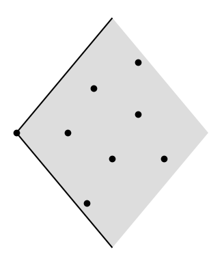
There’s enough information contained in this minimal representation to enable construction of a complete tiling.
All the information required is not directly available in the four vertices. We have to construct a local ‘patch’ by copying and pasting the vertices by the translation vectors, one step in all eight possible directions. The function get_patch() below does the work, returning the local patch vertices as a set. Notably, all the calculations are integer-based.
def get_patch(vs, t1, t2):
  patch = set()
  for k1 in range(-1, 2):
    for k2 in range(-1, 2):
      for v in vs:
        hashcode = vsum(v, vprod(k1, t1), vprod(k2, t2))
        patch.add(hashcode)
  return patch
Using this we can see the four vertices in the context of a repeated pattern.
patch = get_patch(vertices, t1, t2)

ax = base_unit.plot(fc = "#dddddd")
gpd.GeoSeries([get_line(t1)]).plot(ax = ax, color = "k", lw = 0.75)
gpd.GeoSeries([get_line(t2)]).plot(ax = ax, color = "k", lw = 0.75)
gpd.GeoSeries([get_point(v) for v in patch]) \
  .plot(ax = ax, color = "lightgrey")
gpd.GeoSeries([get_point(v) for v in vertices]) \
  .plot(ax = ax, color = "k")
ax.set_axis_off()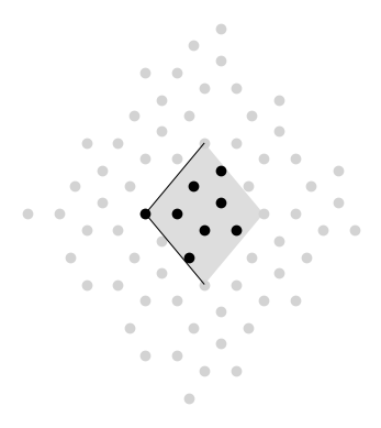
Next, we check for each vertex which other vertices in the local patch are neighbours along a tile edge. If two vertices are separated by one of the 12 unit vectors then they must be neighbours, since all edges in the tiling are one of those vectors, and again, we can carry out this test using only precise integer arithmetic.
The function get_star() below iterates over all 12 vectors checking if when added to the vertex being tested they reach another vertex in the local patch. If so, the index position of the vector is appended to the ‘star’ (it will become clear why it’s call a star in a moment).
def get_star(v, patch):
  star = []
  for k in range(12):
    candidate = vsum(v, BASE_COORDS[k])
    if candidate in patch:
      star.append(k)
  return star
The figure below shows the combined ‘stars’ of all four vertices, and highlights one of them in red.
ax = base_unit.plot(fc = "#dddddd")
gpd.GeoSeries([get_point(v) for v in patch]) \
  .plot(ax = ax, color = "lightgrey")
stars = []
for i, v in enumerate(vertices):
  stars.append(get_star(v, patch))
  color = "r" if i == len(vertices) - 1 else "k"
  gpd.GeoSeries([get_point(v)]).plot(ax = ax, color = color)
  gpd.GeoSeries([get_line(BASE_COORDS[i], v) for i in stars[-1]]) \
    .plot(ax = ax, color = color)
  ax.set_axis_off()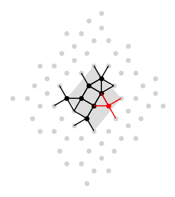
Note that stars are stored only as integers, not complex vectors:
stars[[0, 4, 7, 10],
[2, 6, 8, 11],
[2, 5, 7, 10],
[1, 4, 8, 11],
[0, 2, 5, 8],
[1, 3, 5, 8, 10],
[2, 4, 7, 9, 11],
[1, 4, 6, 10]]The sequence of gaps between the integers in each vertex star tells us the angle at that position, which in turn tells us which kind of polygon it is. A gap of 2 corresponds to 60º and hence a triangle, 3 is 90º hence a square, 4 is 120º hence a hexagon, and 5 is 150º hence a dodecagon.
The gap_to_n_sides() function does this translation.
def gap_to_n_sides(gap):
  k = abs(gap)
  return ( 3 if k == 2
     else  4 if k == 3
     else  6 if k == 4
     else 12 if k == 5
     else gap_to_n_sides(12 - k) if k > 6
     else None)
We’re almost there now.
The functions in the cell below assemble a list of all the tiles (faces) at every vertex. Again, we don’t have to do any floating point calculations. Each face is a sequence of integer 4-tuples, only converted to floating point when we need to plot them.
def get_face(v, heading, n_sides):
  J = 12 // n_sides
  face = [v]
  for angle in range(0, 12, J):
    p = vsum(face[-1], BASE_COORDS[(heading + angle) % 12])
    face.append(p)
  return face[:-1]

def star_to_faces(star, v):
  faces = []
  for left, right in zip(star, [*star[1:], star[0]], strict = True):
    n = gap_to_n_sides((right - left) % 12)
    faces.append(get_face(v, left, n))
  return faces

faces = []
for star, v in zip(stars, vertices):
  faces.extend(star_to_faces(star, v))
ax = base_unit.plot(fc = "#cccccc")
gpd.GeoSeries([get_polygon(f) for f in faces]) \
  .plot(ax = ax, fc = "#ff000030", ec = "k", lw = 0.5)
# gpd.GeoSeries(get_line(t1)).plot(ax = ax, color = "k")
# gpd.GeoSeries(get_line(t2)).plot(ax = ax, color = "k")
ax.set_axis_off()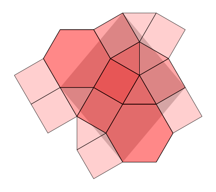
As can be seen in the picture, there are a couple of remaining issues. First, because some tiles are incident at more than one of the vertices, we get multiple copies of them. Second, some tiles clearly lie outside the repeating unit, or mostly outside it, and are not required to generate the repeating tiled pattern. We resolve those issues in the next section.
To resolve these issues, as we build the minimal set of tiles we check to see (i) if we’ve already generated the tile in question, and (ii) if its centroid lies inside the repeating area defined by the translation vectors.
Taking the latter first, a couple more functions are required. This involves some simple matrix mathematics. I’ll spare you the details, but in essence we are checking if a given point lies in the space defined by any combination \(x\mathbf{t}_1 + y\mathbf{t}_2\) such that both \(x\) and \(y\) are in the range 0 to 1.7
def change_base(a, t1, t2):
  det = t1[0] * t2[1] - t1[1] * t2[0]
  d1 =   a[0] * t2[1] -  a[1] * t2[0]
  d2 =  t1[0] *  a[1] - t1[1] *  a[0]
  return d1 / det, d2 / det

def is_in_parallelogram(p, t1, t2):
  U = change_base(to_euclidean(p), to_euclidean(t1), to_euclidean(t2))
  return ((U[0] >= -1e-4) and (U[0] < 1 - 1e-4) and
          (U[1] >= -1e-4) and (U[1] < 1 - 1e-4))
The other aspect to this step as set out in the cell below, that may seem a little odd, is that we keep track of already added tiles, by storing already added tile centroids scaled by a factor of six. This ensures that all tile centroids have integer coordinates, which makes checking and comparing them more reliable. We do have to remember that they have been scaled by six when checking if they fall in the translation vector parallelogram, but that’s easy enough to do.
All this has been put together in the code cell below, where we loop over the vertices, get their stars, get the polygons around the stars, and retain those polygons only if we haven’t already retained them and their centroid lies inside the translation vectors parallelogram.
tiles = []
centroids = set()
for vertex in vertices:
  star = get_star(vertex, patch)
  faces = star_to_faces(star, vertex)
  for face in faces:
    # scale by 6 to ensure integer 4-tuple
    # and remember to downscale below for testing
    centroid = tuple(int(6 * p / len(face)) for p in vsum(*face))
    if centroid not in centroids and \
        is_in_parallelogram(vprod(1/6, centroid), t1, t2):
      centroids.add(centroid)
      tiles.append(face)
And here’s the result.
ax = base_unit.plot(fc = "#dddddd")
gpd.GeoSeries([get_polygon(tile) for tile in tiles]) \
  .plot(ax = ax, fc = "#ff000030", ec = "k")
gpd.GeoSeries([get_point(v) for v in vertices]) \
  .plot(ax = ax, color = "k")
ax.set_axis_off()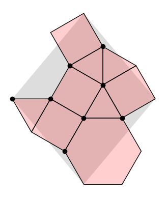
I’m doing all this to extend the range of tilings available in weavingspace, so it’s necessary for my purposes to convert this set of tiles to a weavingspace.TileUnit. Here’s how that works in practice (without getting into too much of the nitty-gritty).
t = wsp.TileUnit()
t.tiles = gpd.GeoDataFrame(
  geometry = gpd.GeoSeries(
    gpd.GeoSeries([get_polygon(tile) for tile in tiles])),
  data = {"tile_id": list("abcdefghi")}, crs = 3857)
t.setup_vectors(to_euclidean(t1), to_euclidean(t2))
t.prototile = t.get_prototile_from_vectors()
t._setup_regularised_prototile(True)
t = t.transform_scale(100, 100)

t.plot(r = 2, r_alpha = 1, cmap = "tab20c",
  show_prototile = False, show_reg_prototile = False, show_ids = False)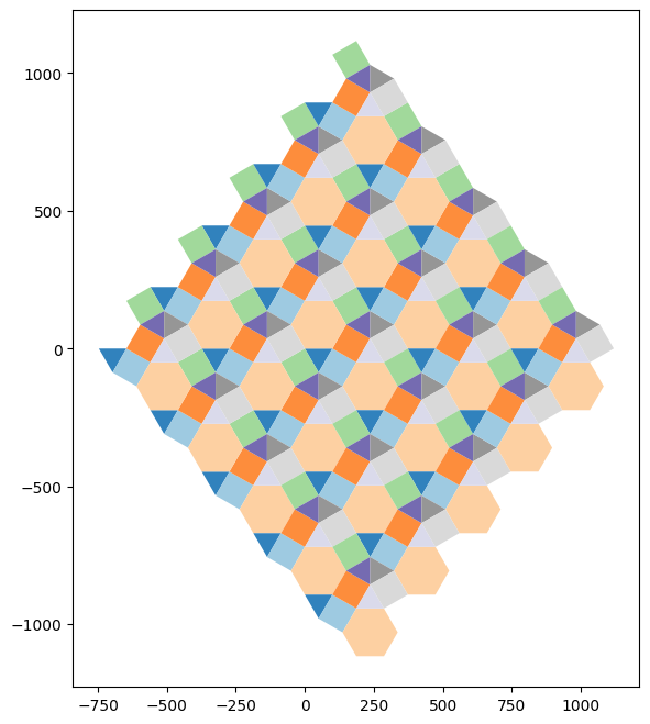
weavingspace using this approach
So far, this code remains in the experimental branch of weavingspace.
Three example tilings from the catalogues produced by the Soto Sanchéz team, alongside their dual tilings generated with the experimental weavingspace code are shown below. I have implemented determination of the dual tilings in keeping with the integer 4-tuples approach.
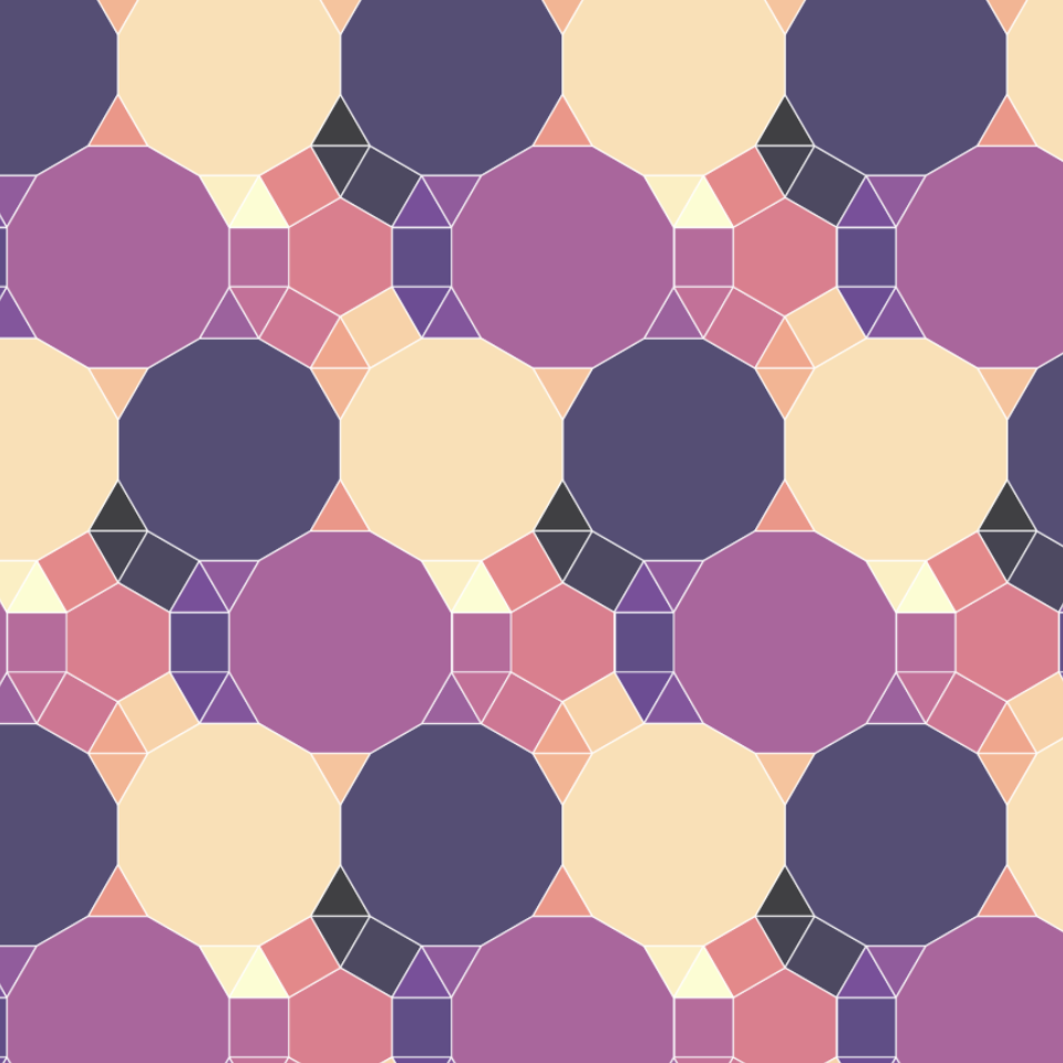
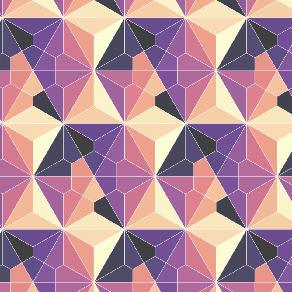
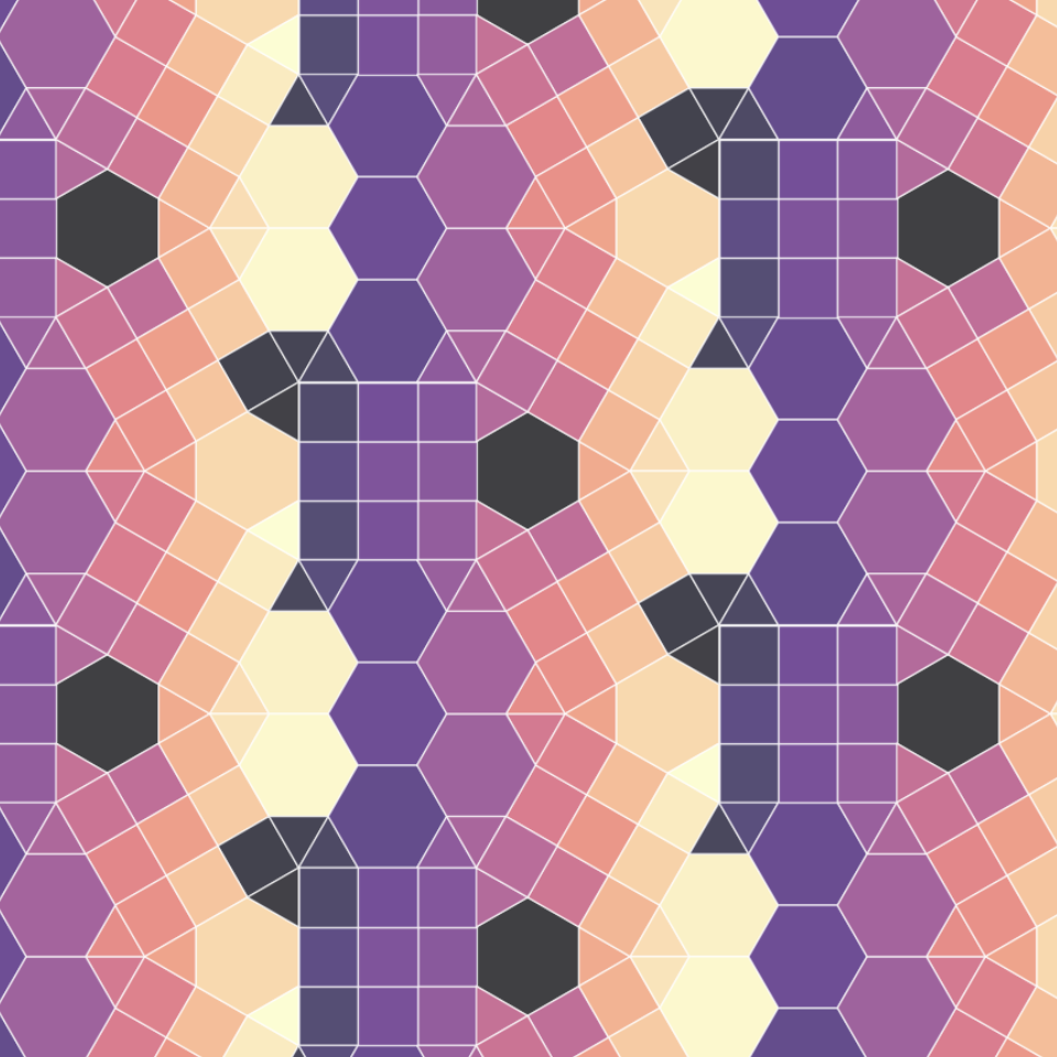
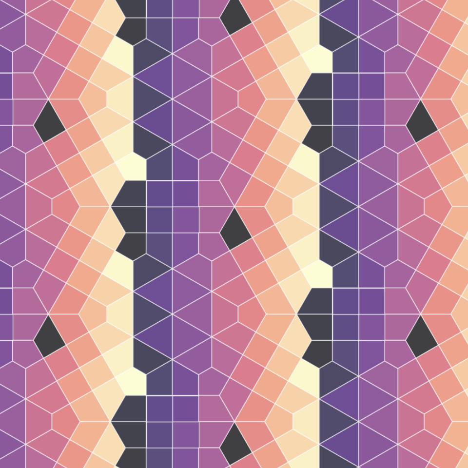
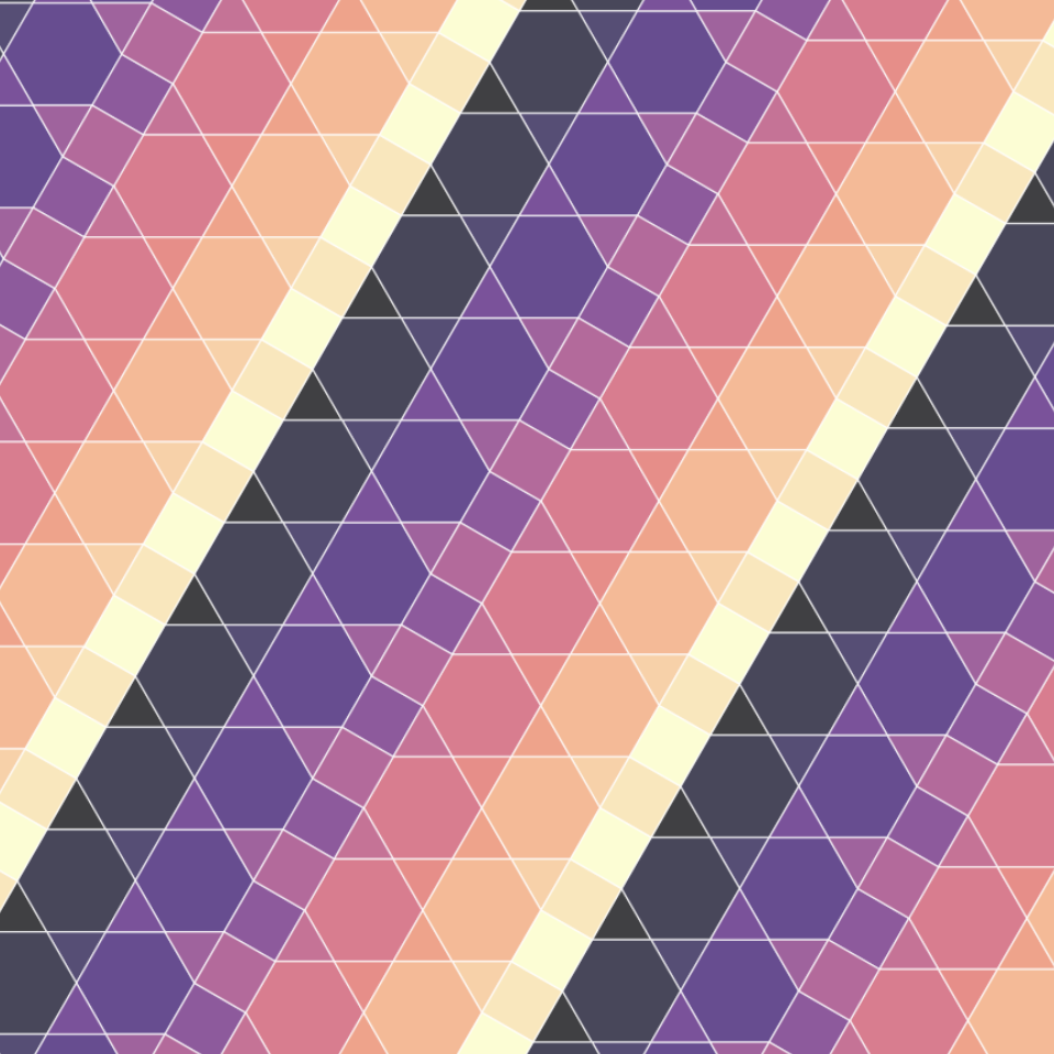
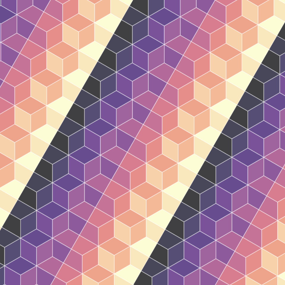
weavingspace using this approach.
As an exercise in the triumph of a data structure and algorithms over doing things in more immediately obvious ways (as mentioned at the top “making a bunch of polygons, then translating and rotating them into position”) this approach takes some beating.
There is something deeply pleasing (to me at least) about how all the pieces of this approach come together. It’s particularly nice not dealing with floating point calculations and the seemingly never ending edge cases they produce. Even in the context of the weavinspace project where many of the hundreds of tilings this method makes available will likely never be used, I’ve found working through the process of putting this code together very rewarding. I hope this outline of how it works has been an interesting read.

Somehow defined…↩︎
There is also a nice Observable notebook implementation here.↩︎
Not hard, and a useful learning process.↩︎
That many tilings creates its own issues of how to navigate and categorise them coherently, but that’s a nice problem to have.↩︎
This bald statement is obviously not a proof, but you can trust me on this… I’m sure it’s mathematically provable, but also, I have hand-coded a lot of these patterns in the last couple of years: it’s definitely true.↩︎
The bane of my life, and of any computation requiring precision geometry.↩︎
This is a floating point test and given all my experiences with weavingspace it makes me nervous!↩︎