(Not) a map of (not) polygons

The Bridges conference series is one of those things I’d like to have got around to when I was still being paid to be an academic. The work presented there lies at the intersection of art and mathematics. I’ve had reason to read papers on the conference archive and if you have even a passing interest in this sort of thing I recommend you do the same.

Anyway, on a recent poke around the archive I came across this paper by Kerry Mitchell:

Mitchell K. 2021. Iterated averaging of polygon vertices. In Proceedings of Bridges 2021: Mathematics, Art, Music, Architecture, Culture, ed. D Swart, F Farris, and E Torrence, 197–204. Phoenix, Arizona: Tessellations Publishing.

As the title makes clear, this paper presents a procedure where consecutive vertices of a polygon are iteratively averaged to produce a series of polygons. Overlaying the resulting polygons makes pretty pictures.

Needless to say, on encountering this I implemented it in Netlogo. You can download that model here if you’re interested, but R is perhaps a more generally useful language, so I thought I’d make some code to make the pictures in R also. And since today is Day 3 of the 30 Day Map Challenge themed ‘Polygons’ and this process makes lots of (not really) polygons and ~~maps~~ plots them, well… why not?

One important caveat is that these aren’t really polygons, because, as we’ll see, they’re tangled up messes of points connected. The edges intersect, and they generally fail any st_is_valid() tests for that reason. We don’t really care about this, because what we’re interested in is making pretty pictures, but it bears mentioning before anyone gets mad at me for calling these things polygons.

The code

As usual, some packages:

Code

library(dplyr)
library(sf)
library(pracma)
library(ggplot2)
library(gganimate)
library(patchwork)

set.seed(0)

1: Useful additional matrix functions.
2: ggplot animations.

The core procedures in iteratively averaging the vertices of a polygon are (i) averaging consecutive vertices¹, and (ii) recentring and rescaling the resulting polygon so that it doesn’t collapse to a point (more on that rabbithole in a moment).

Averaging consecutive corners

Because sf is a thin wrapper around matrices, it’s more convenient to do the manipulations of vertices based on a two-column matrix of the corners of a polygon, than on an sf polygon.

Code

average_corners <- function(m, x = 0.5) {
  m |>
    rbind(m[1, ]) |>
    apply(2, conv, c(x, 1 - x)) |>
    head(-1) |>
    tail(-1)
}

1: Append a copy of the first row of the matrix to the end of the matrix.
2: pracma::conv is a convenient way to average consecutive values in each column of the matrix.
3: The head and tail operations clip the matrix back to its original size so we don’t unintentionally add extra corners.

Here’s an example of this function in operation:

Code

m <- 1:10 |> matrix(ncol = 2, byrow = TRUE)
m

     [,1] [,2]
[1,]    1    2
[2,]    3    4
[3,]    5    6
[4,]    7    8
[5,]    9   10

Code

m |> average_corners()

     [,1] [,2]
[2,]    2    3
[3,]    4    5
[4,]    6    7
[5,]    8    9
[6,]    5    6

Note in particular how the last row in the result is the average of the last row and first row of the original matrix. The x parameter in average_corners() allows for making the new corners closer to the first or last corner of each pair, although we won’t use that here.

Rescaling and recentring a polygon

Next, some functions to recentre and rescale the resulting polygons. If we don’t do this then polygons will collapse to a point.

Iterated averaging of the corners of a polygon is a process, almost but not quite the same as the mice problem which posits the question of what pattern we get if mice each position at the corner of a regular polygon head towards one another at constant speed. Well… not quite towards one another, but towards where they think the mouse they are pursuing will be by the time they get there. The result is a sequence of copies of the original polygon decreasing in size, and with the mice following logarithmic spiral curves.

Turns out this is a bit a rabbithole. Such pursuit problems started out as ‘the problem of the three dogs’ posed by Lucas in 1877, and have been of interest (inevitably) in military contexts where they relate to questions of how to aim missiles at moving targets.² Less militaristically,³ pursuit problems also arise in coordinating autonomous vehicles to conform to desired formations or patterns, as in drone light shows.

Anyway, to recentre and rescale polygons (again, handled as a two-column matrix of points) we have the following function.

Code

get_centre <- function(m) {
  m |>
    apply(2, range) |>
    apply(2, mean)
}

mean_distance_to_centre <- function(m, centre) {
  (m - centre)^2 |>
    apply(1, sum) |>
    sqrt() |>
    mean()
}

recentre <- function(m, r = 1) {
  centre <- m |> get_centre()
  d <- mean_distance_to_centre(m, centre)
  (m - centre) * r / d + centre
}

1: Get the minimum and maximum coordinate in each column.
2: Take the mean to arrive at a centre location.
3: Squared differences to the centre in x and y.
4: Sum the squares, and…
5: … take the square root to get the distances.
6: Return the mean distance.
7: This function uses the other two to recentre and rescale the points in a matrix to a constant mean distance to centre specified by the r parameter.

Converting a matrix to a polygon

We eventually want to convert these matrices to polygons, so we need this function:

Code

matrix_as_polygon <- function(m) {
  rbind(m, m[1, ]) |>
    list() |>
    st_polygon()
}

1: st_polygon requires the first vertex to be repeated.

Making a sequence of polygons

Finally, we can put all these together to get a collection of polygons starting from a random collection of points and iteratively averaging the corners.

Code

get_polygons <- function(n_sides, n_iterations = n_sides * 2, x = 0.5) {
  m <-
    matrix(rnorm(2 * n_sides), ncol = 2) |>
    recentre()
  m_list <- list(m)
  for (i in 1:n_iterations) {
    m_list[[i + 1]] <-
      m_list[[i]] |>
      average_corners(x = x) |>
      recentre()
  }
  m_list |>
    lapply(matrix_as_polygon) |>
    cbind() |>
    st_as_sfc() |>
    data.frame() |>
    st_sf()
}

Results

The first few polygons will be very messy, so it makes sense to drop a few, for our purposes.

Code

drop_frames <- 50
gdf <- get_polygons(200, 500) |>
  slice(-(1:drop_frames))

And finally we can plot one. These are really pretty if we draw the polygon unfilled, using a low opacity colour.

Code

ggplot(gdf) +
  geom_sf(fill = NA, colour = "#00000010") +
  theme_void()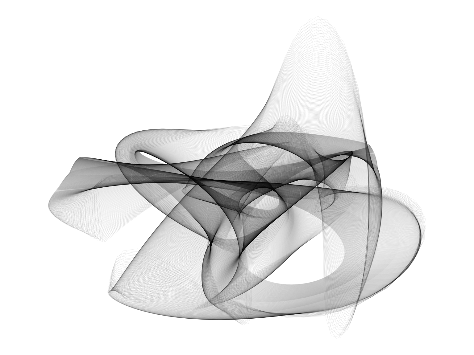

Figure 1: An example picture based on overlaying steps in the iterative corner averaging process.

The process animated

Using gganimate::animate we can animate the sequence of polygons to get a better feel for the process.

Code

anim <- ggplot(gdf |> mutate(t = row_number())) +
  geom_sf(fill = NA, colour = "black") +
  transition_manual(t) +
  theme_void()

animate(anim, nframes = nrow(gdf), fps = 25)

More pretty pictures

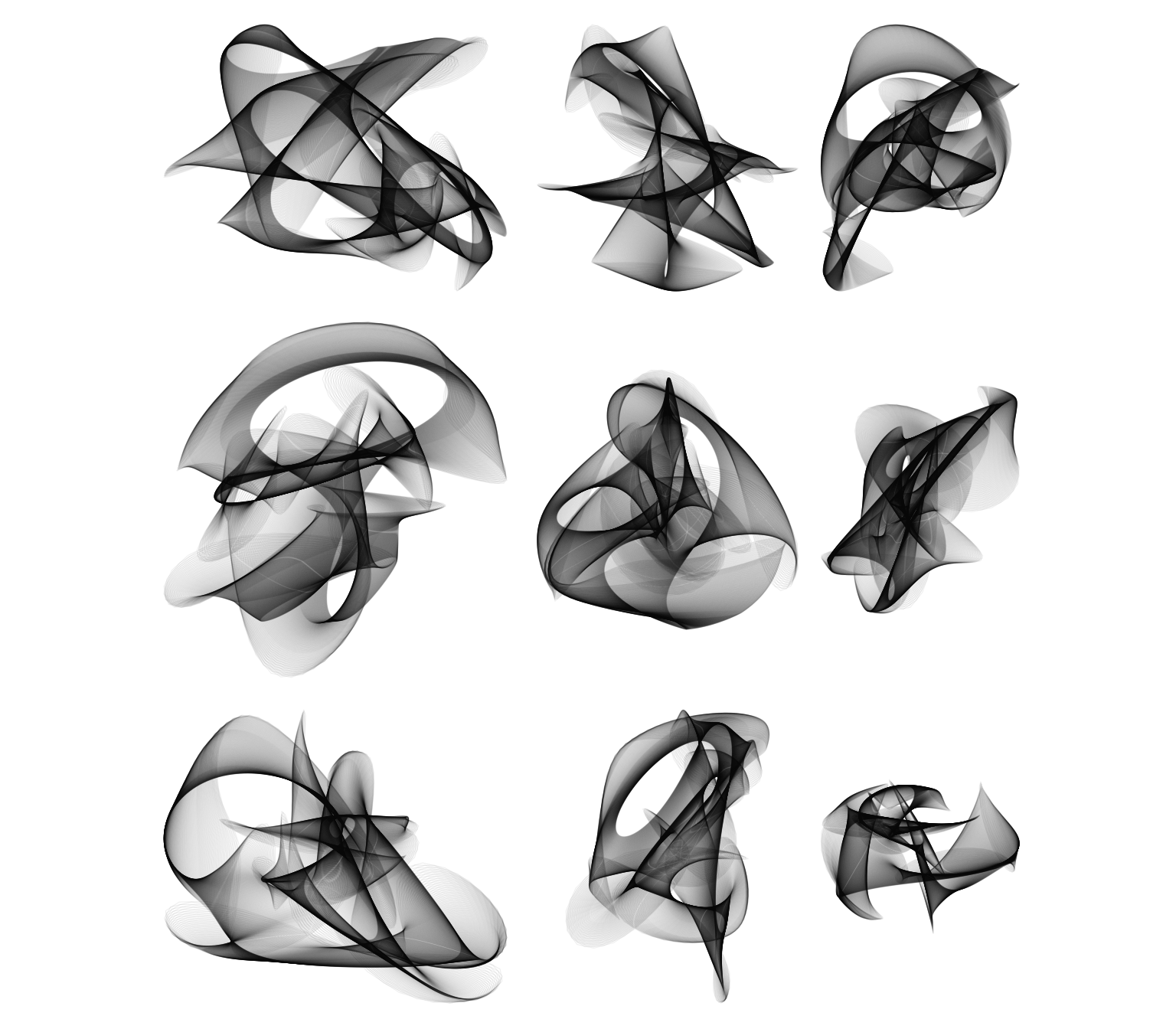
Finally, here are some more examples.

Footnotes

Duh.↩︎
Absolutely the most crazily named ‘problem’ in this realm is the homicidal chauffeur problem, so named (according to wikipedia) as an “unclassified proxy for missile defence” problems!↩︎
Although given recent developments in drone warfare perhaps not very much less so…↩︎